Lab 9: Linear Regression Analysis

Author

Instructor Name

Published

September 6, 2025

Student Name:

Introduction: Linear Regression Analysis

This laboratory focuses on linear regression analysis, emphasizing model building, interpretation, and diagnostic checking. We will explore simple linear regression concepts through practical applications using real and simulated datasets, with particular attention to regression assumptions and model validation.

Learning Objectives

Upon completion of this laboratory, students will be able to:

  • Understand and apply the assumptions of simple linear regression
  • Fit and interpret linear regression models using R’s lm() function
  • Perform comprehensive diagnostic checks using residual analysis
  • Assess model fit and identify potential violations of assumptions
  • Apply regression analysis to real-world educational datasets
  • Compare regression models across different scenarios

Time Allocation (Total: 100 minutes)

  • Part 1: Regression Fundamentals and Assumptions (35 minutes)
  • Part 2: Model Building and Interpretation (35 minutes)
  • Part 3: Diagnostic Analysis and Validation (30 minutes)

Part 1: Regression Fundamentals and Assumptions

1.1 Understanding Linear Regression

Linear regression models the relationship between a response variable (Y) and one or more predictor variables (X) using a linear equation:

Y=β0+β1X+ϵY = \beta_0 + \beta_1 X + \epsilon

Where: - β0\beta_0 is the intercept (expected Y when X = 0) - β1\beta_1 is the slope (change in Y per unit change in X) - ϵ\epsilon is the error term (random variation)

1.2 Key Regression Assumptions

For valid inference in linear regression, four key assumptions must be met:

  1. Linearity: Relationship between X and Y is linear
  2. Independence: Observations are independent of each other
  3. Homoscedasticity: Constant variance of errors across X values
  4. Normality: Residuals are approximately normally distributed

1.3 Data Import and Preparation

# Load datasets for regression analysis
# Data URL: https://math214.netlify.app/data/Lab9/TestScore.csv
TestScore <- read.csv("../data/Lab9/TestScore.csv")
# Data URL: https://math214.netlify.app/data/Lab9/FA.csv
FA <- read.csv("../data/Lab9/FA.csv")


# TestScore Dataset Preview
glimpse(TestScore)
Rows: 64
Columns: 7
$ T1            <dbl> 72.3, 65.8, 79.1, 48.6, 12.4, 42.8, 74.6, 88.9, 54.2, 82…
$ T2            <dbl> 85.2, 82.4, 86.5, 79.8, 28.7, 55.3, 83.9, 95.2, 70.8, 75…
$ T3            <dbl> 81.7, 75.9, 80.2, 55.7, 8.3, 15.2, 77.8, 89.4, 67.3, 70.…
$ Tave          <dbl> 79.7, 74.7, 81.9, 61.4, 16.5, 37.8, 78.7, 91.2, 64.1, 76…
$ HW            <int> 95, 72, 92, 63, 34, 85, 89, 94, 76, 46, 78, 85, 73, 33, …
$ FinalExam     <int> 78, 68, 52, 58, 12, 39, 76, 79, 51, 65, 57, 69, 75, 49, …
$ CourseAverage <dbl> 83.2, 73.4, 74.1, 62.3, 19.8, 48.2, 79.8, 88.5, 62.4, 67…
# FA Dataset Preview
glimpse(FA)
Rows: 20
Columns: 6
$ X  <int> 10, 8, 13, 9, 11, 14, 6, 4, 12, 7, 5, NA, NA, NA, NA, NA, NA, NA, N…
$ Y1 <dbl> 8.04, 6.95, 7.58, 8.81, 8.33, 9.96, 7.24, 4.26, 10.84, 4.82, 5.68, …
$ Y2 <dbl> 9.14, 8.14, 8.74, 8.77, 9.26, 8.10, 6.13, 3.10, 9.13, 7.26, 4.74, N…
$ Y3 <dbl> 7.46, 6.77, 12.74, 7.11, 7.81, 8.84, 6.08, 5.39, 8.15, 6.42, 5.73, …
$ X4 <int> 8, 8, 8, 8, 8, 8, 8, 19, 8, 8, 8, NA, NA, NA, NA, NA, NA, NA, NA, NA
$ Y4 <dbl> 6.58, 5.76, 7.71, 8.84, 8.47, 7.04, 5.25, 12.50, 5.56, 7.91, 6.89, …
Part 2: Model Building and Interpretation

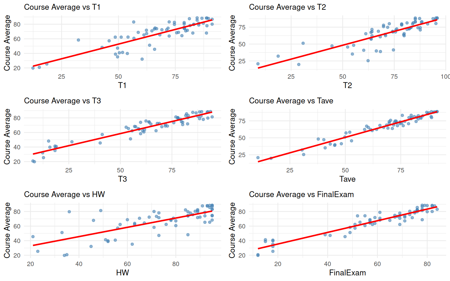
2.1 Simple Linear Regression with Test Score Data

[1] "Scatter Plots in 3x2 Grid:"

2.1 Simple Linear Regression with Test Score Data

[1] "Correlations with Course Average:"
Correlation Coefficients with Course Average
Predictor Correlation
T1 0.8425264
T2 0.8290517
T3 0.9525896
Tave 0.9685652
HW 0.7378745
FinalExam 0.9483872

2.2 Comprehensive Regression Analysis

[1] "Regression Analysis Summary:"
Linear Regression Metrics for All Predictors
Predictor Intercept Slope R_squared RMSE
T1 12.414 0.806 0.710 9.416388
T2 7.137 0.822 0.687 9.775051
T3 25.301 0.663 0.907 5.318825
Tave 5.079 0.913 0.938 4.348643
HW 20.134 0.637 0.544 11.798791
FinalExam 19.441 0.799 0.899 5.543575
[1] "Best predictor: Tave with R-squared: 0.938"

Part 3: Diagnostic Analysis and Validation

3.1 Model Diagnostics for Best Predictor

# Fit best model
best_model <- lm(CourseAverage ~ Tave, data = TestScore)

# Create diagnostic plots using moderndive
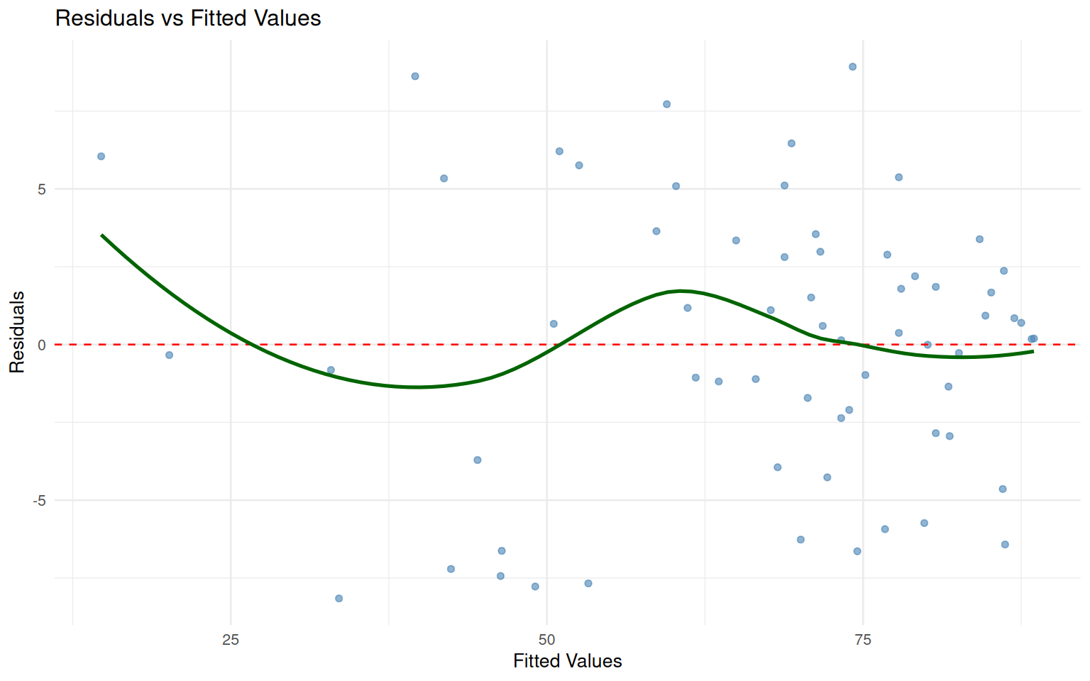
print("Residual Plot:")
[1] "Residual Plot:"
residual_plot <- ggplot(best_model, aes(x = .fitted, y = .resid)) +
  geom_point(alpha = 0.6, color = "steelblue") +
  geom_hline(yintercept = 0, linetype = "dashed", color = "red") +
  geom_smooth(se = FALSE, color = "darkgreen") +
  labs(title = "Residuals vs Fitted Values",
       x = "Fitted Values", y = "Residuals") +
  theme_minimal(base_size = 10)
print(residual_plot)

Residuals vs Fitted Values

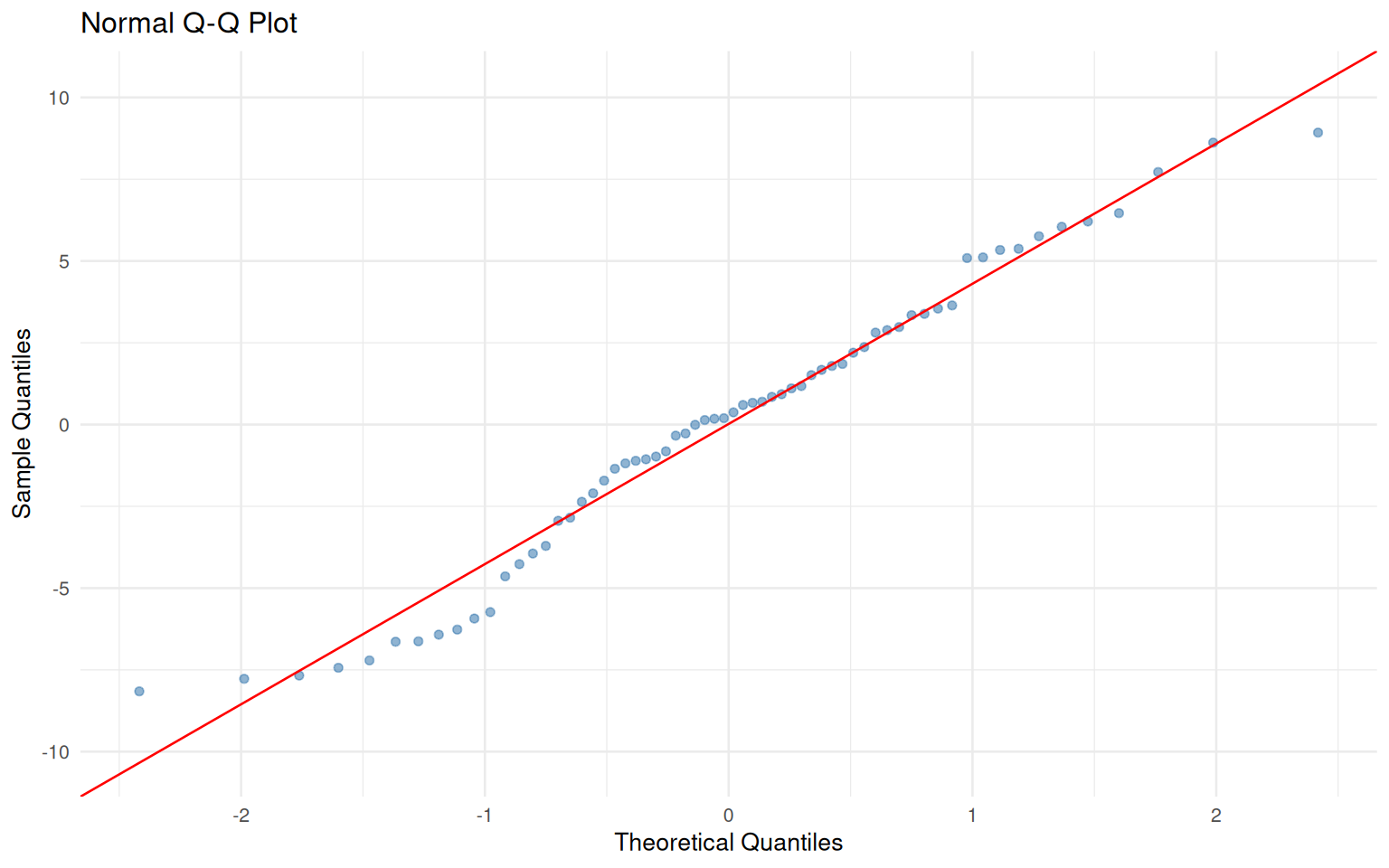
print("Q-Q Plot:")
[1] "Q-Q Plot:"
qq_plot <- ggplot(best_model, aes(sample = .resid)) +
  stat_qq(alpha = 0.6, color = "steelblue") +
  stat_qq_line(color = "red") +
  labs(title = "Normal Q-Q Plot",
       x = "Theoretical Quantiles", y = "Sample Quantiles") +
  theme_minimal(base_size = 10)
print(qq_plot)

Residuals vs Fitted Values

# Additional diagnostics using moderndive
print("Model Diagnostics Summary:")
[1] "Model Diagnostics Summary:"
coef_table <- get_regression_table(best_model)
model_summary <- get_regression_summaries(best_model)

# Create summary table
model_summary_df <- tibble(
  Metric = c("Intercept", "Slope (Tave)", "R-squared", "RMSE"),
  Value = c(
    round(as.numeric(coef_table$estimate[coef_table$term == "intercept"]), 3),
    round(as.numeric(coef_table$estimate[coef_table$term != "intercept"]), 3),
    round(as.numeric(model_summary$r_squared), 3),
    round(as.numeric(model_summary$rmse), 3)
  )
)

knitr::kable(model_summary_df, caption = "Best Model (CourseAverage ~ Tave) Summary")
Best Model (CourseAverage ~ Tave) Summary
Metric Value
Intercept 5.079
Slope (Tave) 0.913
R-squared 0.938
RMSE 4.349
# Get regression points for detailed analysis
regression_points <- get_regression_points(best_model)
print("First few regression points:")
[1] "First few regression points:"
knitr::kable(head(regression_points), caption = "First 6 Regression Points")
First 6 Regression Points
ID CourseAverage Tave CourseAverage_hat residual
1 83.2 79.7 77.826 5.374
2 73.4 74.7 73.262 0.138
3 74.1 81.9 79.834 -5.734
4 62.3 61.4 61.123 1.177
5 19.8 16.5 20.139 -0.339
6 48.2 37.8 39.581 8.619
# Normality test
shapiro_test <- shapiro.test(residuals(best_model))
print(paste("Shapiro-Wilk normality test p-value:",
            format.pval(shapiro_test$p.value, digits = 3)))
[1] "Shapiro-Wilk normality test p-value: 0.182"

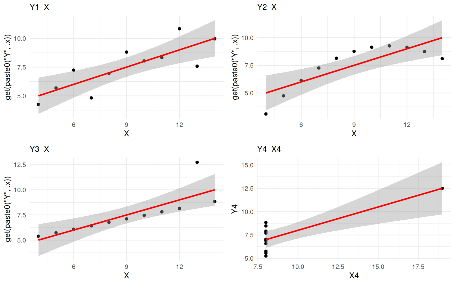
3.2 Anscombe’s Quartet Analysis

[1] "Anscombe's Quartet Regression Statistics:"
Identical Regression Metrics Across Anscombe’s Quartet
Dataset Intercept Slope R_squared RMSE
Y1_X 3.000 0.5 0.667 1.118550
Y2_X 3.001 0.5 0.666 1.119102
Y3_X 3.002 0.5 0.666 1.118286
Y4_X4 3.002 0.5 0.667 1.117729
[1] "Anscombe's Quartet Plots in 2x2 Grid:"

3.2 Anscombe's Quartet Analysis

Assessment (Total: 50 points)

Section A: Formative Understanding (15 points)

A1. Explain the four key assumptions of simple linear regression and why each is important for valid inference. Provide specific examples of what happens when each assumption is violated. (4 points)

A2. Interpret the regression coefficients from the best predictor model (CourseAverage ~ Tave). What do the intercept and slope represent in the context of student performance? (4 points)

A3. Define R-squared and explain what it measures in regression analysis. Provide an example interpretation of an R-squared value of 0.94 in the context of the test score data. (4 points)

A4. Describe how residual plots help diagnose violations of regression assumptions. What specific patterns would indicate problems with linearity, homoscedasticity, or normality? (3 points)

Section B: Application and Analysis (20 points)

B1. Using the TestScore dataset, identify which individual test (T1, T2, or T3) is the strongest predictor of CourseAverage. Provide both visual evidence (scatter plots) and quantitative evidence (R-squared values) to support your conclusion. (5 points)

# Your code for B1 here
# Create scatter plots and calculate R-squared for T1, T2, T3

B2. Compare the regression models for Tave and FinalExam as predictors of CourseAverage. Which provides better prediction and why? Consider both statistical measures (R-squared, p-values) and practical implications. (5 points)

# Your code for B2 here
# Compare Tave and FinalExam models

B3. Perform comprehensive diagnostic checking for the best predictor model (CourseAverage ~ Tave). Create residual plots, test for normality, and assess whether regression assumptions appear reasonably met. (5 points)

# Your code for B3 here
# Diagnostic analysis for best model

B4. Analyze Anscombe’s quartet datasets. What do the regression outputs have in common across all four datasets? What important statistical lesson does Anscombe’s quartet illustrate about relying solely on numerical summaries? (5 points)

# Your code for B4 here
# Anscombe's quartet analysis

Section C: Statistical Synthesis (15 points)

C1. Design a research study where linear regression would be appropriate for analyzing educational outcomes. Describe the variables, expected relationship, and how you would validate the regression assumptions. Include specific methods for checking each assumption. (7 points)

C2. Create a comprehensive diagnostic framework for linear regression analysis. Outline the key diagnostic checks, what each check assesses, and what actions should be taken when assumptions appear violated. (4 points)

C3. Discuss the practical implications of regression analysis in educational assessment. How can regression results inform teaching strategies, student support, or curriculum development? Provide specific examples based on the test score analysis. (4 points)

Submission Guidelines:

  • Complete R Markdown document with all code and analysis
  • Proper execution of all regression analyses and diagnostic checks
  • Comprehensive interpretation of regression results in context
  • Professional writing with clear analytical narrative
  • Appropriate use of ggplot for all visualizations
  • Knitted HTML document submitted via designated platform