Skip to main content

Lab 8: Hypothesis Testing for Small Samples

Student Name:

Introduction: Small Sample Hypothesis Testing

This laboratory focuses on hypothesis testing procedures for small samples ($n < 30$), emphasizing the critical importance of normality assessment. When sample sizes are small, the Central Limit Theorem no longer provides protection, making formal normality testing essential for valid inference.

Learning Objectives

Upon completion of this laboratory, students will be able to:

• Understand the challenges and considerations for small sample hypothesis testing
• Conduct comprehensive normality assessments using Anderson-Darling tests and QQ-plots
• Perform appropriate parametric tests (t-tests) when normality assumptions are met
• Interpret test results in practical contexts with appropriate error analysis
• Select appropriate statistical tests based on sample characteristics

Time Allocation (Total: 75 minutes)

• Part 1: Small Sample Challenges and Normality Assessment (30 minutes)
• Part 2: Parametric Testing for Normal Small Samples (25 minutes)
• Part 3: Practical Applications and Decision Framework (20 minutes)

Part 1: Small Sample Challenges and Normality Assessment

1.1 Navigating Small Sample Challenges

When $n < 30$, the assumptions underlying parametric tests become more sensitive. To ensure valid inference, we must:

1. Conduct thorough normality diagnostics
2. Use appropriate graphical methods for visual assessment
3. Select tests based on distribution characteristics
4. Consider robust alternatives when assumptions are questionable

Small Sample Challenges:

• Increased Sensitivity to Assumptions: Normality assumptions become more influential with $n < 30$
• Central Limit Theorem protection diminishes: CLT no longer provides adequate protection
• Outliers and skewness have greater impact: Individual data points have more influence on results
• Consequences of Normality Violation: Type I error ($\alpha$) inflation, Type II error ($\beta$) increase, biased estimates, invalid inference

1.2 Normality Diagnostics

Q-Q Plots Interpretation:

• Points deviating from the reference line (y = x) suggest non-normality
• Left skew: Points curve below the line at high quantiles
• Heavy tails: Points flare outward at extremes
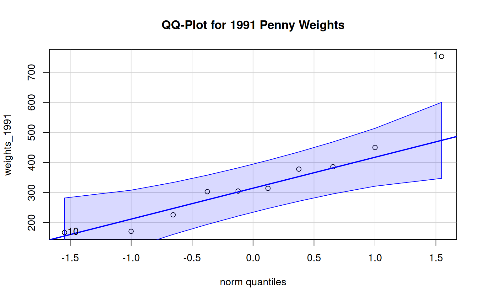
• Use car::qqPlot() for added confidence bands (reject normality if >1 point falls outside bands)

Anderson-Darling Test (nortest::ad.test):

• Null Hypothesis ($H_0$): The data comes from a normal distribution
• Alternative Hypothesis ($H_1$): The data does not come from a normal distribution
• Test Statistic: Weighted quadratic distance between empirical and theoretical CDF
• Typical $\alpha$: 0.05 (5% significance level)

Interpretation:

• p-value $\geq$ 0.05: Fail to reject $H_0$ → insufficient evidence against normality assumption. This does not prove normality, but suggests the test did not detect significant deviations from normality. May proceed with parametric tests cautiously, but always verify with graphical methods.
• p-value $<$ 0.05: Reject $H_0$ → strong evidence against normality assumption. The data shows significant deviation from a normal distribution. Consider non-parametric alternatives or data transformations.

Practical Decision Framework:

• p-value $<$ 0.01: Very strong evidence against normality → definitely use non-parametric methods
• 0.01 $\leq$ p-value $<$ 0.05: Moderate evidence against normality → strongly consider non-parametric methods
• p-value $\geq$ 0.05: Insufficient evidence against normality → may use parametric tests with caution

1.3 Data Import and Preparation

# Load banking data for small sample analysis
# Data URL: https://math214.netlify.app/data/Lab8/banking.csv
banking_data <- read.csv("../data/Lab8/banking.csv")

# Extract variables for analysis
weights_1991 <- banking_data$X1991
weights_1990 <- banking_data$X1990

# Define comprehensive summary function
summarize_data <- function(data, name) {
  ad_test <- ad.test(data)
  list(
    Dataset = name,
    n = length(data),
    Mean = mean(data),
    Median = median(data),
    SD = sd(data),
    AD_p = ad_test$p.value,
    Normal = ad_test$p.value >= 0.05
  )
}

# Apply summary function to datasets
summary_1991 <- summarize_data(weights_1991, "1991 Weights")
summary_1990 <- summarize_data(weights_1990, "1990 Weights")

# Display summary objects
print("1991 Penny Weights Summary:")

[1] "1991 Penny Weights Summary:"

print(summary_1991)

$Dataset
[1] "1991 Weights"

$n
[1] 10

$Mean
[1] 345.3

$Median
[1] 309.5

$SD
[1] 170.1973

$AD_p
[1] 0.1076069

$Normal
[1] TRUE

print("1990 Penny Weights Summary:")

[1] "1990 Penny Weights Summary:"

print(summary_1990)

$Dataset
[1] "1990 Weights"

$n
[1] 10

$Mean
[1] 451.7

$Median
[1] 343

$SD
[1] 336.3196

$AD_p
[1] 0.000704652

$Normal
[1] FALSE

Part 2: Parametric Testing for Normal Small Samples

2.1 T-tests for Normal Small Samples

When normality assumptions are met (based on Anderson-Darling test and QQ-plots), t-tests remain appropriate for small samples:

# Example: Test if 1991 mean weight equals 450g
# First assess normality
ad_1991 <- ad.test(weights_1991)
print("Anderson-Darling Test for 1991 Weights:")

[1] "Anderson-Darling Test for 1991 Weights:"

print(ad_1991)

    Anderson-Darling normality test

data:  weights_1991
A = 0.5634, p-value = 0.1076

# Visual assessment
qqPlot(weights_1991, main = "QQ-Plot for 1991 Penny Weights")

[1]  1 10

# Test selection and execution based on normality
if(ad_1991$p.value >= 0.05) {
  print("Proceeding with t-test (normality assumption met):")
  t_test_1991 <- t.test(weights_1991, mu = 450)
  print(t_test_1991)
} else {
  print("Proceeding with Sign test (normality assumption violated):")
  sign_test_1991 <- SIGN.test(weights_1991, md = 450)
  print(sign_test_1991)
}

[1] "Proceeding with t-test (normality assumption met):"

    One Sample t-test

data:  weights_1991
t = -1.9453, df = 9, p-value = 0.08359
alternative hypothesis: true mean is not equal to 450
95 percent confidence interval:
 223.5482 467.0518
sample estimates:
mean of x 
    345.3 

Part 3: Practical Applications and Decision Framework

3.1 Complete Hypothesis Testing Framework

For small samples, follow this enhanced eight-step framework:

1. Problem Description: State hypotheses in context

2. Symbolic Formulation: $H_0: \mu = \mu_0$, $H_1: \mu \neq, >, < \mu_0$

3. Significance Level: Specify $\alpha$ (typically 0.05)

4. Normality Assessment:

   • Anderson-Darling test (formal)
   • QQ-plot (visual)
   • If $p \geq 0.05$: proceed with t-test
   • If $p < 0.05$: consider alternative approaches

5. Test Selection: Choose t-test if normality confirmed

6. Test Execution: Compute test statistic and p-value

7. Conclusion: State decision in context with effect size

8. Error Analysis: Discuss potential Type I/II errors

3.2 Built-in Datasets for Practice

# Load built-in datasets
# Puromycin dataset for enzyme kinetics analysis
data(Puromycin)
untreated_rates <- Puromycin[Puromycin$state == "untreated", ]$rate

# Pressure dataset for temperature analysis
data(pressure)
temperatures <- pressure$temperature

# Apply summary function to built-in datasets
puro_summary <- summarize_data(untreated_rates, "Puromycin (untreated)")
pressure_summary <- summarize_data(temperatures, "Pressure")

# Display summary objects
print("Puromycin Untreated Rates Summary:")

[1] "Puromycin Untreated Rates Summary:"

print(puro_summary)

$Dataset
[1] "Puromycin (untreated)"

$n
[1] 11

$Mean
[1] 110.7273

$Median
[1] 115

$SD
[1] 36.52695

$AD_p
[1] 0.8726029

$Normal
[1] TRUE

print("Pressure Temperature Summary:")

[1] "Pressure Temperature Summary:"

print(pressure_summary)

$Dataset
[1] "Pressure"

$n
[1] 19

$Mean
[1] 180

$Median
[1] 180

$SD
[1] 112.5463

$AD_p
[1] 0.8326693

$Normal
[1] TRUE

# Test if untreated reaction rates differ from 100
ad_puro <- ad.test(untreated_rates)
print("Anderson-Darling Test for Puromycin:")

[1] "Anderson-Darling Test for Puromycin:"

print(ad_puro)

    Anderson-Darling normality test

data:  untreated_rates
A = 0.1888, p-value = 0.8726

if(ad_puro$p.value >= 0.05) {
  print("Proceeding with t-test:")
  t_test_puro <- t.test(untreated_rates, mu = 100)
  print(t_test_puro)
} else {
  print("Proceeding with Sign test:")
  sign_test_puro <- SIGN.test(untreated_rates, md = 100)
  print(sign_test_puro)
}

[1] "Proceeding with t-test:"

    One Sample t-test

data:  untreated_rates
t = 0.97403, df = 10, p-value = 0.353
alternative hypothesis: true mean is not equal to 100
95 percent confidence interval:
  86.18813 135.26641
sample estimates:
mean of x 
 110.7273 

# Test if temperatures differ from 150
ad_pressure <- ad.test(temperatures)
print("Anderson-Darling Test for Pressure:")

[1] "Anderson-Darling Test for Pressure:"

print(ad_pressure)

    Anderson-Darling normality test

data:  temperatures
A = 0.21132, p-value = 0.8327

if(ad_pressure$p.value >= 0.05) {
  print("Proceeding with t-test:")
  t_test_pressure <- t.test(temperatures, mu = 150)
  print(t_test_pressure)
} else {
  print("Proceeding with Sign test:")
  sign_test_pressure <- SIGN.test(temperatures, md = 150)
  print(sign_test_pressure)
}

[1] "Proceeding with t-test:"

    One Sample t-test

data:  temperatures
t = 1.1619, df = 18, p-value = 0.2605
alternative hypothesis: true mean is not equal to 150
95 percent confidence interval:
 125.7544 234.2456
sample estimates:
mean of x 
      180 

Assessment (Total: 50 points)

Section A: Formative Understanding (15 points)

A1. Explain the challenges of hypothesis testing with small samples ($n < 30$). Discuss why normality assessment becomes critical and what consequences arise from violating normality assumptions in small samples. (4 points)

A2. Describe the Anderson-Darling test for normality. What are its null and alternative hypotheses? How should the results be interpreted, and what specific actions should be taken based on different p-value outcomes? (4 points)

A3. Compare and contrast hypothesis testing for large samples ($n \geq 30$) versus small samples ($n < 30$). Focus on the role of the Central Limit Theorem and the importance of normality assessment. (4 points)

A4. Discuss the enhanced eight-step hypothesis testing framework for small samples. Explain how normality assessment integrates into the framework and why this step is crucial for valid inference. (3 points)

Section B: Application and Analysis (20 points)

B1. Test whether the mean penny weight in 1991 differs from 450g using $\alpha = 0.05$. First conduct comprehensive normality assessment (Anderson-Darling test and QQ-plot), then select and execute the appropriate test following the eight-step framework. (5 points)

# Normality assessment
ad_result <- ad.test(weights_1991)
ad_result

# QQ-plot
qqPlot(weights_1991)

# Test selection and execution
if(ad_result$p.value >= 0.05) {
  t.test(weights_1991, mu = 450)
} else {
  SIGN.test(weights_1991, md = 450)
}

B2. Test whether the 1990 median penny weight exceeds 350g using $\alpha = 0.05$. Conduct proper normality assessment and select the appropriate test method. Compare your approach and results with B1. (5 points)

# Normality assessment
ad_result <- ad.test(weights_1990)
ad_result

# QQ-plot
qqPlot(weights_1990)

# Test selection and execution
if(ad_result$p.value >= 0.05) {
  t.test(weights_1990, mu = 350, alternative = "greater")
} else {
  SIGN.test(weights_1990, md = 350, alternative = "greater")
}

B3. A biologist claims untreated enzyme reaction rates average 100 nmol/min. Using the Puromycin dataset (untreated group), test this claim with $\alpha = 0.05$. First assess normality, then select the appropriate test and interpret your results in the biological context. (5 points)

# Extract untreated reaction rates
untreated_rates <- Puromycin[Puromycin$state == "untreated", ]$rate

# Normality assessment
ad_result <- ad.test(untreated_rates)
ad_result

# QQ-plot
qqPlot(untreated_rates)

# Test selection and execution
if(ad_result$p.value >= 0.05) {
  t.test(untreated_rates, mu = 100)
} else {
  SIGN.test(untreated_rates, md = 100)
}

B4. Generate comprehensive summary statistics tables for all three datasets (1991 weights, 1990 weights, Puromycin untreated rates). Include measures of central tendency, variability, and normality test results. Discuss how these descriptive statistics inform your hypothesis testing decisions. (5 points)

# Generate summaries using the predefined summarize_data function
summary_1991 <- summarize_data(weights_1991, "1991 Weights")
summary_1990 <- summarize_data(weights_1990, "1990 Weights")
summary_puro <- summarize_data(untreated_rates, "Puromycin Rates")

# Display results
summary_1991
summary_1990
summary_puro

Section C: Statistical Synthesis (15 points)

C1. Create a comprehensive decision framework (200-250 words) for selecting appropriate hypothesis tests based on sample size and distribution characteristics. Include specific guidance for when t-tests are appropriate for small samples and when alternative approaches should be considered. (7 points)

C2. Design a practical scenario where a researcher might encounter non-normal small sample data. Explain the challenges this presents and discuss the importance of transparent reporting of assumption checks in research publications. (4 points)

C3. Develop a simulation study design to evaluate the performance of different hypothesis testing approaches with small samples from various non-normal distributions. Outline the methodology, evaluation criteria, and expected findings. (4 points)

Submission Guidelines:

• Complete R Markdown document with all code and analysis
• Proper execution of all hypothesis tests following the eight-step framework
• Comprehensive normality assessments with both formal tests and graphical methods
• Professional writing with clear analytical narrative and interpretation
• Appropriate test justifications based on normality assessment results
• Knitted HTML document submitted via designated platform