Lab 3: Discrete Random Variables and Probability Distributions

Author

Instructor Name

Published

September 25, 2025

Student Name:

Introduction: Discrete Probability Distributions

This laboratory introduces fundamental discrete probability distributions and their applications in statistical modeling. We will explore three key discrete distributions, Uniform, Binomial, and Poisson, through theoretical understanding, computational implementation, and practical interpretation.

Time Allocation (Total: 100 minutes)

Part 1: Discrete Uniform Distribution (30 minutes)
Part 2: Binomial Distribution Analysis (35 minutes)
Part 3: Poisson Distribution and Distribution Matching (35 minutes)

Part 1: Discrete Uniform Distribution

1.1 R Distribution Functions Overview

R provides comprehensive functions for working with probability distributions through four key prefixes:

R Distribution Function Prefixes

Prefix	Purpose	Example Functions
`r`	Random sample generation	`rnorm`, `rbinom`, `runif`
`d`	Density function	`dnorm`, `dbinom`, `dunif`
`p`	Cumulative distribution function	`pnorm`, `pbinom`, `punif`
`q`	Quantile function	`qnorm`, `qbinom`, `qunif`

1.2 Discrete Uniform Distribution Theory

The discrete uniform distribution dU(a,b) assigns equal probability to all integers between a and b inclusive.

# Theoretical properties of dU(1,30)
a <- 1
b <- 30
uniform_probs <- rep(1/(b - a + 1), b - a + 1)
uniform_df <- tibble(
  Value = a:b,
  Probability = uniform_probs,
  Cumulative = cumsum(uniform_probs)
)

head(uniform_df, 10)

# A tibble: 10 × 3
   Value Probability Cumulative
   <int>       <dbl>      <dbl>
 1     1      0.0333     0.0333
 2     2      0.0333     0.0667
 3     3      0.0333     0.1   
 4     4      0.0333     0.133 
 5     5      0.0333     0.167 
 6     6      0.0333     0.2   
 7     7      0.0333     0.233 
 8     8      0.0333     0.267 
 9     9      0.0333     0.3   
10    10      0.0333     0.333

1.3 Probability Calculations

Calculating probabilities using both theoretical formulas and R functions.

Probability Calculations for dU(1,30)

P(5 < X ≤ 7) = 0.0667
P(X > 5) = 0.8333
P(X ≥ 5) = 0.8667
P(5 ≤ X ≤ 7) = 0.1

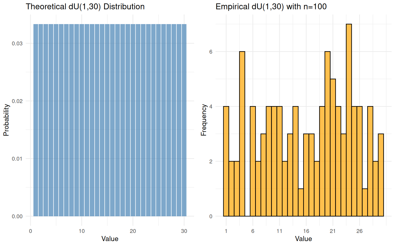
1.4 Random Sampling and Distribution Comparison

Generating random samples and comparing empirical distributions to theoretical expectations.

Part 2: Binomial Distribution Analysis

2.1 Binomial Distribution Fundamentals

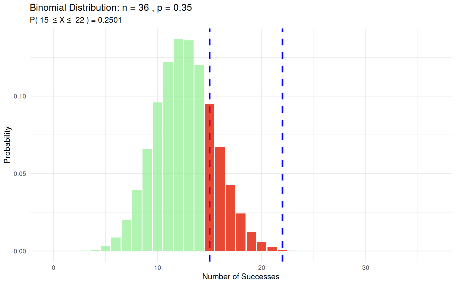
The binomial distribution models the number of successes in n independent trials.

# Binomial distribution visualization function
binom_plotter <- function(n, p, lb, ub) {
  data <- tibble(
    x = 0:n,
    px = dbinom(0:n, n, p)
  )
  
  ggplot(data, aes(x, px)) + 
    geom_col(fill = "lightgreen", alpha = 0.7) +
    geom_vline(xintercept = c(lb, ub), linetype = "dashed", color = "blue", size = 1) +
    geom_col(data = data[data$x >= lb & data$x <= ub,], 
             aes(x, px), fill = "red", alpha = 0.7) +
    labs(title = paste("Binomial Distribution: n =", n, ", p =", p),
         subtitle = paste("P(", lb, " ≤ X ≤ ", ub, ") =",
                         round(pbinom(ub, n, p) - pbinom(lb - 1, n, p), 4)),
         x = "Number of Successes", y = "Probability") +
    theme_minimal(base_size = 10)
}

# Example: Bin(36, 0.35) with P(15 ≤ X ≤ 22)
binom_plotter(36, 0.35, 15, 22)

2.2 Probability Boundary Cases

Understanding how inequality signs affect probability calculations.

Binomial Probability Boundary Cases (n=36, p=0.35)

P(X = 15) = 0.095
P(15 < X ≤ 22) = 0.155
P(15 ≤ X < 22) = 0.2492
P(X ≥ 22) = 0.0012

2.3 Distribution Shape Analysis

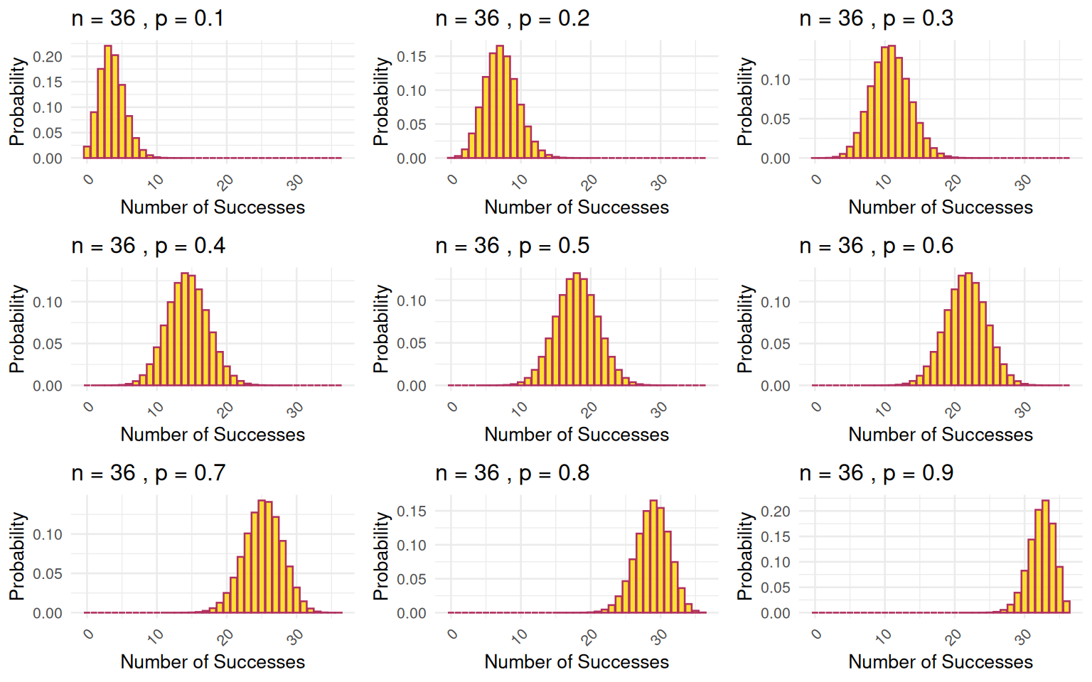
Examining how parameter p affects binomial distribution shape.

# Binomial distribution shape analysis
n <- 36
p_values <- seq(0.1, 0.9, by = 0.1)

binomial_plots <- lapply(p_values, function(p) {
  data <- tibble(x = 0:n, prob = dbinom(0:n, n, p))
  ggplot(data, aes(x, prob)) +
    geom_col(fill = "gold", color = "maroon", alpha = 0.8) +
    labs(title = paste("n =", n, ", p =", p),
         x = "Number of Successes", y = "Probability") +
    theme_minimal(base_size = 10) +
    theme(axis.text.x = element_text(angle = 45, hjust = 1))
})

grid.arrange(grobs = binomial_plots, ncol = 3)

Part 3: Poisson Distribution and Distribution Matching

3.1 Poisson Distribution Applications

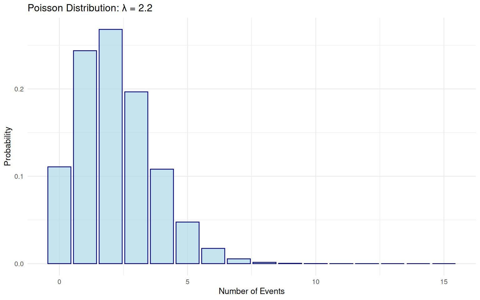
The Poisson distribution models rare events occurring in fixed intervals.

Poisson Distribution Calculations (λ = 2.2)

P(X > 3) = 0.1806
P(2.2 < X < 5.1) = 0.3524

# Poisson distribution visualization
lambda <- 2.2
poisson_data <- tibble(x = 0:15, prob = dpois(0:15, lambda))

ggplot(poisson_data, aes(x, prob)) +
  geom_col(fill = "lightblue", color = "navy", alpha = 0.7) +
  labs(title = paste("Poisson Distribution: λ =", lambda),
       x = "Number of Events", y = "Probability") +
  theme_minimal(base_size = 10)

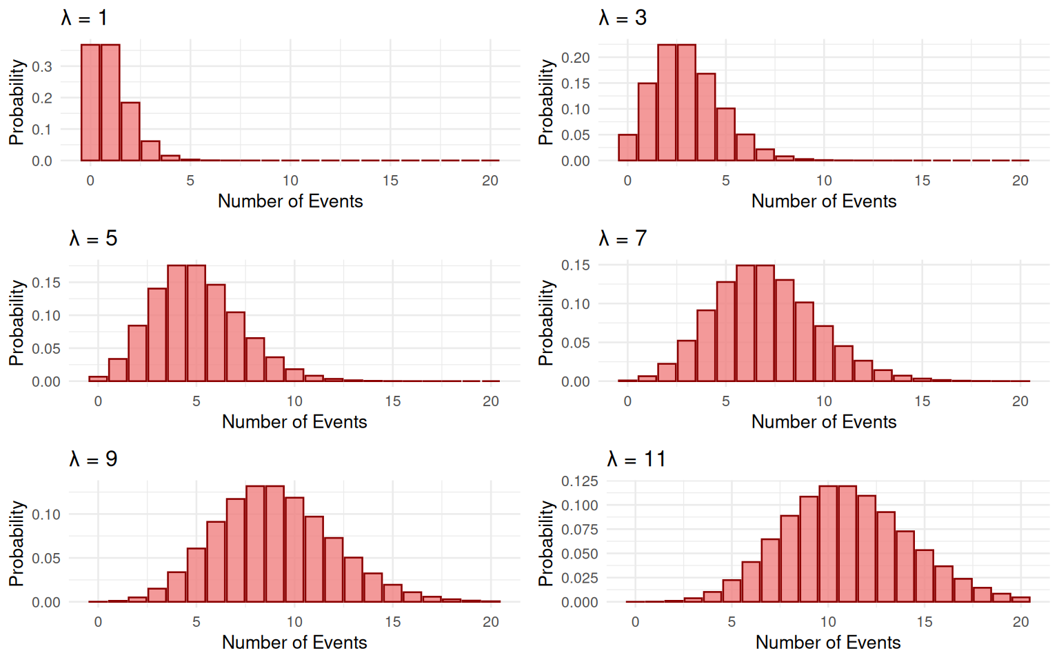
Poisson Distribution Calculations (λ = 2.2)

3.2 Poisson Distribution Shape Analysis

Examining how λ affects Poisson distribution characteristics.

# Poisson distribution shape analysis
lambda_values <- c(1, 3, 5, 7, 9, 11)

poisson_plots <- lapply(lambda_values, function(lambda) {
  data <- tibble(x = 0:20, prob = dpois(0:20, lambda))
  ggplot(data, aes(x, prob)) +
    geom_col(fill = "lightcoral", color = "darkred", alpha = 0.8) +
    labs(title = paste("λ =", lambda),
         x = "Number of Events", y = "Probability") +
    theme_minimal(base_size = 10)
})

grid.arrange(grobs = poisson_plots, ncol = 2)

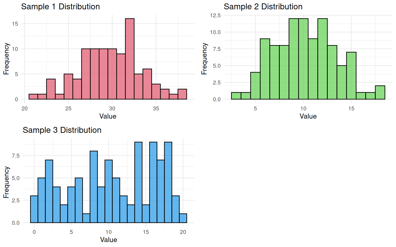
3.3 Distribution Matching Exercise

Using descriptive statistics to match empirical samples to theoretical distributions.

# Load sample data for distribution matching
# Data URL: https://math214.netlify.app/data/Lab3/Samples2.csv
data0 <- read.csv("../data/Lab3/Samples2.csv")

# Visual examination of samples
sample_plots <- list()
for (i in 1:3) {
  sample_plots[[i]] <- ggplot(data0, aes(x = .data[[paste0("Sample_", i)]])) +
    geom_histogram(binwidth = 1, fill = i+1, alpha = 0.7, color = "black") +
    labs(title = paste("Sample", i, "Distribution"),
         x = "Value", y = "Frequency") +
    theme_minimal(base_size = 10)
}

grid.arrange(grobs = sample_plots, ncol = 2)

Assessment (Total: 50 points)

Section A: Formative Understanding (15 points)

A1. Explain the differences between R’s four distribution function prefixes (r, d, p, q) and provide examples of when each would be used in statistical analysis. (4 points)

A2. Compare and contrast the discrete uniform, binomial, and Poisson distributions. What real-world phenomena would each distribution be appropriate for modeling? (4 points)

A3. Discuss how sample size affects the resemblance between empirical histograms and theoretical probability distributions. Use examples from the uniform distribution analysis to support your explanation. (4 points)

A4. Analyze how the parameter p affects the shape of the binomial distribution. For what values of p is the distribution symmetric, and why does this occur? (3 points)

Section B: Coding Proficiency (20 points)

B1. Generate three random samples of size 1000 from dU(1,30) and create histograms for each sample. Overlay the theoretical distribution on each histogram and discuss the results. (4 points)

# Your code here

B2. For the binomial distribution with n=36 and p=0.35, calculate the following probabilities: P(X ≥ 17), P(X ≥ 17.4), and P(X ≥ 17.6). Explain any differences in the results. (4 points)

# Your code here

B3. Create a comprehensive visualization showing the Poisson distribution for λ values from 1 to 9. Arrange the plots in a grid and analyze how the distribution shape changes with increasing λ. (4 points)

# Your code here

B4. Calculate descriptive statistics (mean, variance, range) for each sample in Samples2.csv and use these statistics to match each sample to its theoretical distribution (U(0,20), Bin(50,0.6), or Pois(10)). (4 points)

# Your code here

B5. Investigate the relationship between λ and distribution skewness in the Poisson distribution. Determine for what values of λ the distribution appears right-skewed and provide quantitative evidence. (4 points)

# Your code here

Section C: Statistical Synthesis (15 points)

C1. Write a comprehensive report (200-250 words) discussing the practical applications of discrete probability distributions in real-world scenarios. Include specific examples for each distribution type and explain how parameter choices affect model appropriateness. (7 points)

C2. Design a complete statistical analysis plan for a research study that could utilize all three discrete distributions (uniform, binomial, Poisson). Specify the research questions, data collection methods, and analytical approaches for each distribution. (4 points)

C3. Reflect on the limitations of using discrete distributions for modeling continuous phenomena. What considerations should researchers keep in mind when choosing between discrete and continuous distributions? (4 points)

Submission Guidelines:

Complete R Markdown document with all code and outputs
Properly formatted visualizations and statistical summaries
Professional writing with clear analytical narrative
Knitted HTML document submitted via designated platform