# Creating numeric objects
population_maryland <- 4.2  # Millions
state_count <- 50

# Creating sequence objects
state_ranks <- 1:50
population_vector <- seq(0.5, 40, by = 0.5)

# Performing arithmetic operations
total_population_estimate <- population_maryland * state_count
scaled_ranks <- state_ranks * 2Lab 0: Introduction to R Programming
Student Name:
Introduction: Foundations of Statistical Computing
This laboratory introduces the fundamental principles of R programming with emphasis on statistical data manipulation, visualization, and interpretation.
Learning Objectives
Upon completion of this laboratory, students will be able to:
- Create and manipulate R objects using appropriate syntax
- Import and explore structured datasets
- Perform data filtering, transformation, and summarization operations
- Generate meaningful visualizations using ggplot2
- Interpret statistical patterns and relationships in context
- Document analytical processes using R Markdown
Time Allocation (Total: 100 minutes)
- Part 1: Foundational Concepts (30 minutes)
- Part 2: Data Manipulation Techniques (35 minutes)
- Part 3: Visualization and Interpretation (35 minutes)
Part 1: Foundational R Programming Concepts
1.1 Objects and Basic Operations
R utilizes objects to store data and functions to perform operations. Understanding object creation and manipulation forms the basis of statistical computing.
1.2 Data Import and Initial Exploration
Statistical analysis begins with data acquisition. We will examine demographic data for US states from the 1970s.
# Importing the dataset
# Data URL: https://math214.netlify.app/data/Lab0/states.csv
states_data <- read.csv("../data/Lab0/states.csv")
# Dataset dimensions
dim(states_data)[1] 50 12# Variable names
names(states_data) [1] "Name" "Abbreviation" "Region" "Division" "Population"
[6] "Income" "Illiteracy" "LifeExp" "Murder" "HS_Grad"
[11] "Frost" "Area" head(states_data, 3) Name Abbreviation Region Division Population Income Illiteracy
1 Alabama AL South East South Central 3615 3624 2.1
2 Alaska AK West Pacific 365 6315 1.5
3 Arizona AZ West Mountain 2212 4530 1.8
LifeExp Murder HS_Grad Frost Area
1 69.05 15.1 41.3 20 50708
2 69.31 11.3 66.7 152 566432
3 70.55 7.8 58.1 15 113417The dataset contains 50 observations with 12 variables including state names, regional classifications, population estimates, economic indicators, and educational metrics.
1.3 Basic Data Manipulation with Base R
Traditional R syntax provides multiple approaches for data subsetting and filtering.
# Extracting specific observations and variables
states_data[1, ]  # First observation
Name Abbreviation Region Division Population Income Illiteracy
1 Alabama AL South East South Central 3615 3624 2.1
LifeExp Murder HS_Grad Frost Area
1 69.05 15.1 41.3 20 50708states_data[, 2] # Second variable [1] "AL" "AK" "AZ" "AR" "CA" "CO" "CT" "DE" "FL" "GA" "HI" "ID" "IL" "IN" "IA"
[16] "KS" "KY" "LA" "ME" "MD" "MA" "MI" "MN" "MS" "MO" "MT" "NE" "NV" "NH" "NJ"
[31] "NM" "NY" "NC" "ND" "OH" "OK" "OR" "PA" "RI" "SC" "SD" "TN" "TX" "UT" "VT"
[46] "VA" "WA" "WV" "WI" "WY"states_data[1:5, 2:5] # Submatrix Abbreviation Region Division Population
1 AL South East South Central 3615
2 AK West Pacific 365
3 AZ West Mountain 2212
4 AR South West South Central 2110
5 CA West Pacific 21198# Conditional filtering
maryland_info <- states_data[states_data$Name == "Maryland", ]
southern_states <- subset(states_data, Region == "South")
# Working with specific variables
state_names <- states_data$Name
population_values <- states_data$PopulationPart 2: Modern Data Manipulation with Tidyverse
2.1 Introduction to Tidyverse Principles
The tidyverse ecosystem provides coherent tools for data science workflows, emphasizing readability and reproducibility.
Functions and Pipes
A function is a named set of instructions: inputs go in, an output comes out. For example, mean(c(2, 4, 6)) returns 4. Many functions accept optional arguments, such as na.rm = TRUE, which tells R to ignore missing values.
A pipe (|>) passes the result on its left into the first argument of the next function. This makes a multi-step analysis read from left to right instead of nesting many parentheses.
# Three equivalent ways to compute a mean
mean(c(2, 4, 6))
[1] 4c(2, 4, 6) |> mean()[1] 4# A short data pipeline using functions and pipes
states_data |>
filter(Region == "South") |>
summarise(
avg_population = mean(Population),
count_states = n()
) avg_population count_states
1 4208.125 16# Using native pipes for data workflows
states_data |>
filter(Region == "South") |>
select(Name, Population, Income, Illiteracy) |>
arrange(desc(Population)) Name Population Income Illiteracy
1 Texas 12237 4188 2.2
2 Florida 8277 4815 1.3
3 North Carolina 5441 3875 1.8
4 Virginia 4981 4701 1.4
5 Georgia 4931 4091 2.0
6 Tennessee 4173 3821 1.7
7 Maryland 4122 5299 0.9
8 Louisiana 3806 3545 2.8
9 Alabama 3615 3624 2.1
10 Kentucky 3387 3712 1.6
11 South Carolina 2816 3635 2.3
12 Oklahoma 2715 3983 1.1
13 Mississippi 2341 3098 2.4
14 Arkansas 2110 3378 1.9
15 West Virginia 1799 3617 1.4
16 Delaware 579 4809 0.92.2 Advanced Data Transformation
Creating calculated variables and performing grouped operations enables sophisticated analytical capabilities.
# Creating new calculated variables
states_data <- states_data |>
  mutate(
    population_density = Population / Area,
    income_per_capita = Income / Population
  )

# Grouped summarization
regional_summary <- states_data |>
  group_by(Region) |>
  summarise(
    avg_population = mean(Population),
    avg_income = mean(Income),
    total_states = n(),
    min_illiteracy = min(Illiteracy),
    max_illiteracy = max(Illiteracy)
  )

regional_summary
# A tibble: 4 × 6
Region avg_population avg_income total_states min_illiteracy max_illiteracy
<chr> <dbl> <dbl> <int> <dbl> <dbl>
1 North Ce… 4803 4611. 12 0.5 0.9
2 Northeast 5495. 4570. 9 0.6 1.4
3 South 4208. 4012. 16 0.9 2.8
4 West 2915. 4703. 13 0.5 2.22.3 Comprehensive Data Analysis with Restaurant Data
Expanding our analytical toolkit with a different dataset provides comparative context.
# Importing restaurant tipping data
# Data URL: https://math214.netlify.app/data/Lab0/tips.csv
tips_data <- read.csv("../data/Lab0/tips.csv")

# Data transformation and analysis
tips_analysis <- tips_data |>
  mutate(
    tip_percentage = (tip / total_bill) * 100,
    tip_per_person = tip / size
  ) |>
  group_by(day, time, sex) |>
  summarise(
    avg_bill = mean(total_bill),
    avg_tip_pct = mean(tip_percentage),
    avg_tip_per_person = mean(tip_per_person),
    n_observations = n()
  ) |>
  arrange(day, time, desc(avg_tip_pct))

tips_analysis
# A tibble: 11 × 7
# Groups: day, time [6]
day time sex avg_bill avg_tip_pct avg_tip_per_person n_observations
<chr> <chr> <chr> <dbl> <dbl> <dbl> <int>
1 Fri Dinner Female 14.3 19.9 1.40 5
2 Fri Dinner Male 23.5 13.0 1.35 7
3 Fri Lunch Female 13.9 20.0 1.25 4
4 Fri Lunch Male 11.4 17.4 1.27 3
5 Sat Dinner Female 19.7 15.6 1.27 28
6 Sat Dinner Male 20.8 15.2 1.19 59
7 Sun Dinner Female 19.9 18.2 1.19 18
8 Sun Dinner Male 21.9 16.2 1.22 58
9 Thur Dinner Female 18.8 16.0 1.5 1
10 Thur Lunch Male 18.7 16.5 1.26 30
11 Thur Lunch Female 16.6 15.7 1.08 31Part 3: Data Visualization and Statistical Interpretation
3.1 Exploratory Visualization with ggplot2
Visual representation facilitates pattern recognition and hypothesis generation in statistical analysis.
# Population distribution visualization
ggplot(states_data, aes(x = Population)) +
  geom_histogram(binwidth = 2000, fill = "steelblue", color = "black", alpha = 0.7) +
  labs(title = "Distribution of State Populations (1970s)",
       subtitle = "Histogram showing frequency of population values across US states",
       x = "Population (thousands)",
       y = "Frequency") +
  theme_minimal(base_size = 10)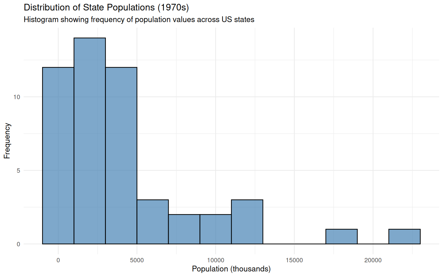
3.2 Multivariate Relationships
Examining relationships between variables reveals underlying statistical patterns.
# Income vs Illiteracy by Region
ggplot(states_data, aes(x = Income, y = Illiteracy, color = Region, size = Population)) +
  geom_point(alpha = 0.7) +
  labs(title = "Income and Illiteracy Relationship by Region",
       subtitle = "Bubble plot showing economic and educational indicators across US regions",
       x = "Income (per capita, dollars)",
       y = "Illiteracy Rate (%)",
       color = "Region",
       size = "Population (thousands)") +
  theme_minimal(base_size = 10) +
  scale_size_continuous(range = c(2, 8))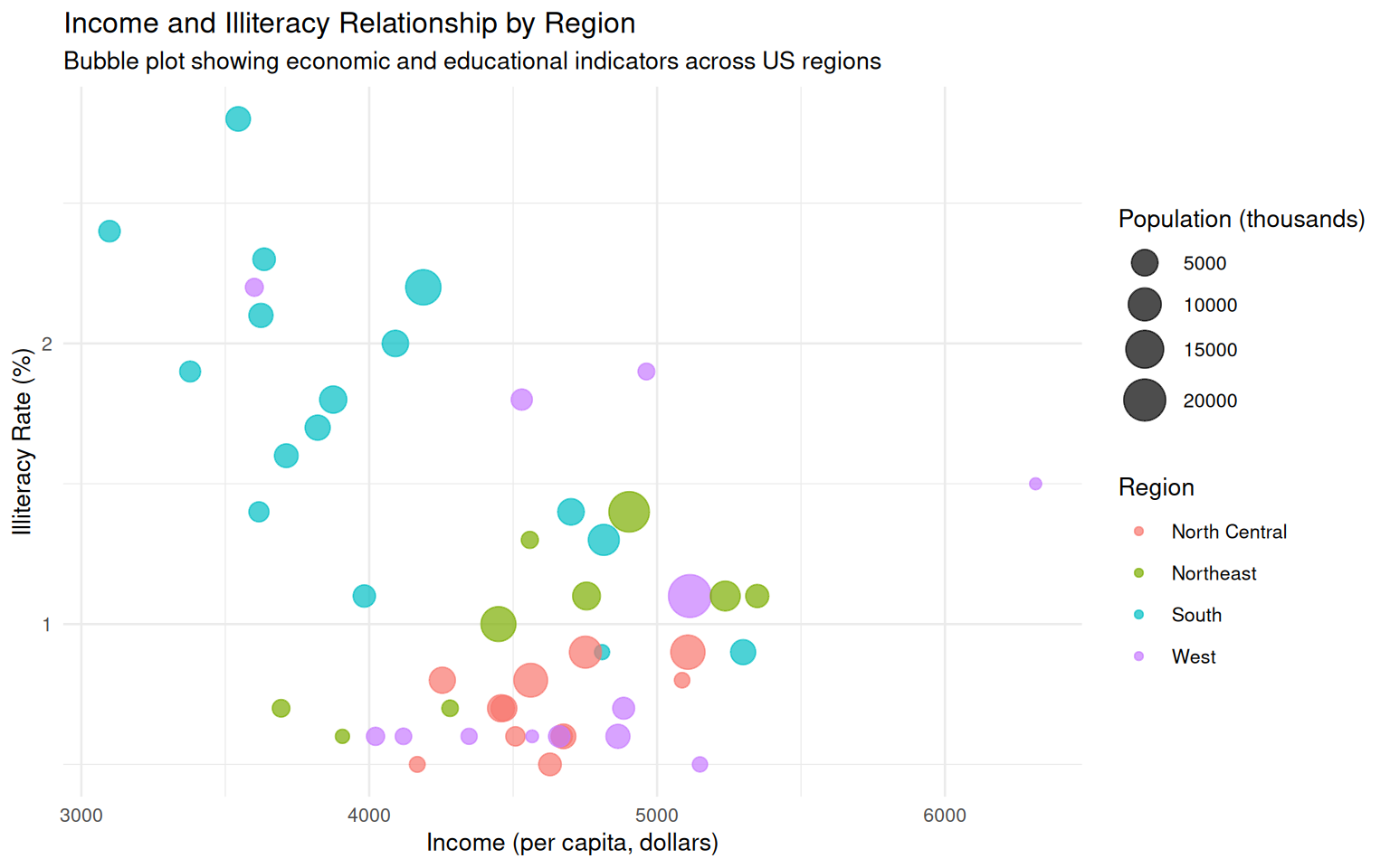
3.3 Comparative Analysis with Tipping Data
# Tip analysis by time and day
ggplot(tips_data, aes(x = total_bill, y = tip, color = time)) +
  geom_point(alpha = 0.6) +
  facet_wrap(~day) +
  labs(title = "Tip Amounts by Total Bill and Service Time",
       subtitle = "Scatterplot showing relationship between bill amount and tips across different days",
       x = "Total Bill (dollars)",
       y = "Tip Amount (dollars)",
       color = "Service Time") +
  theme_minimal(base_size = 10)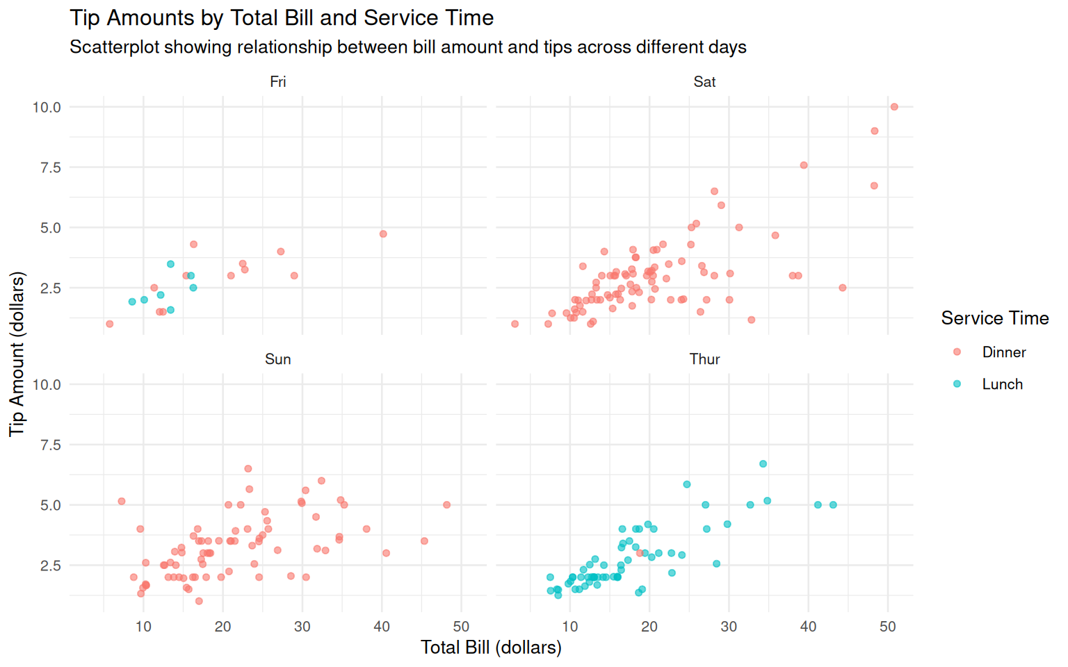
Assessment (Total: 50 points)
Section A: Formative Understanding (15 points)
A1. Describe the difference between base R indexing (e.g., data[1,]) and tidyverse filtering (e.g., filter(data, condition)) approaches. Which method provides greater readability for complex operations? (3 points)
A2. Explain the purpose of the mutate() function in data transformation. Provide an example of creating a meaningful calculated variable from the states dataset. (3 points)
A3. Interpret the relationship shown in the Income vs Illiteracy visualization. What statistical pattern is evident, and how might regional differences contribute to this pattern? (4 points)
A4. Discuss the importance of data visualization in statistical analysis. How do the histograms and scatterplots created in this lab facilitate understanding of the underlying distributions and relationships? (5 points)
Section B: Coding Proficiency (20 points)
B1. Create a vector containing even numbers from 2 to 50 using appropriate R syntax. (2 points)
B2. Import the states.csv dataset and display the names of states with population greater than 10,000 and located in the Northeast region. (4 points)
# Your code here
# states_data <- read.csv("https://math214.netlify.app/data/Lab0/states.csv")
B3. Using the tips dataset, calculate the average tip percentage for lunch vs dinner service. Which service time receives higher percentage tips? (4 points)
# Your code here
# tips_data <- read.csv("https://math214.netlify.app/data/Lab0/tips.csv")
B4. Create a new variable in the states dataset representing income per thousand population. Then generate summary statistics of this variable by region. (5 points)
# Your code hereB5. Produce a boxplot visualization showing the distribution of illiteracy rates by region. Provide appropriate labels and formatting. (5 points)
# Your code hereSection C: Statistical Synthesis (15 points)
C1. Based on your analysis of both datasets, write a brief comparative interpretation (150-200 words) discussing the different types of variables (demographic vs behavioral) and their analytical implications. (7 points)
C2. Propose two research questions that could be investigated using the states dataset, specifying the analytical approaches that would be appropriate for each question. (4 points)
C3. Reflect on the limitations of the tipping dataset for making generalizations about restaurant tipping behavior. What additional variables would strengthen such an analysis? (4 points)
Submission Guidelines:
- Complete R Markdown document with all code and outputs
- Properly formatted visualizations and statistical summaries
- Professional writing with clear analytical narrative
- Knitted HTML document submitted via MyClasses