Lab 10: Chi-Square Tests for Categorical Data Analysis
Author
Instructor Name
Published
November 19, 2025
Student Name:
Introduction: Chi-Square Tests for Categorical Data
This laboratory focuses on chi-square tests for analyzing relationships between categorical variables. Chi-square tests are essential statistical tools for examining whether observed frequency distributions differ from expected distributions or whether categorical variables are independent.
Learning Objectives
Upon completion of this laboratory, students will be able to:
Understand the concepts and applications of chi-square tests
Perform chi-square tests of independence for categorical variables
Conduct chi-square goodness-of-fit tests
Interpret chi-square test results and p-values
Check assumptions for chi-square tests
Handle sparse data situations with Fisher’s exact test
Apply chi-square tests to real-world datasets
Communicate statistical findings from categorical data analysis
Time Allocation (Total: 75 minutes)
Part 1: Chi-Square Test Concepts and Assumptions (25 minutes)
Part 2: Test of Independence Applications (30 minutes)
Part 3: Goodness-of-Fit Testing (20 minutes)
Part 1: Chi-Square Test Concepts and Assumptions
1.1 Chi-Square Test Fundamentals
Chi-square tests are used for categorical data analysis and come in two main forms:
Test of Independence: Examines whether two categorical variables are related
Goodness-of-Fit Test: Compares observed frequencies to expected frequencies
Key Concepts:
Contingency Table: A table showing frequency distributions of categorical variables
Expected Frequencies: The frequencies we would expect if the null hypothesis were true
Chi-Square Statistic: Measures the discrepancy between observed and expected frequencies
Degrees of Freedom: Determined by the dimensions of the contingency table
1.2 Assumptions and Conditions
For valid chi-square tests, the following assumptions must be met:
Random Sampling: Data should come from a random sample
Independence: Observations must be independent of each other
Expected Counts: All expected frequencies should be ≥ 5
Categorical Data: Variables must be categorical, not continuous
Expected Counts Condition:
When expected counts < 5, the chi-square approximation may be inaccurate
For 2×2 tables with small expected counts, use Fisher’s exact test
For larger tables, consider combining categories or using exact tests
1.3 Hypothesis Formulation
Test of Independence:
: The two categorical variables are independent
: The two categorical variables are dependent
Goodness-of-Fit Test:
: The observed frequencies match the expected distribution
: The observed frequencies do not match the expected distribution
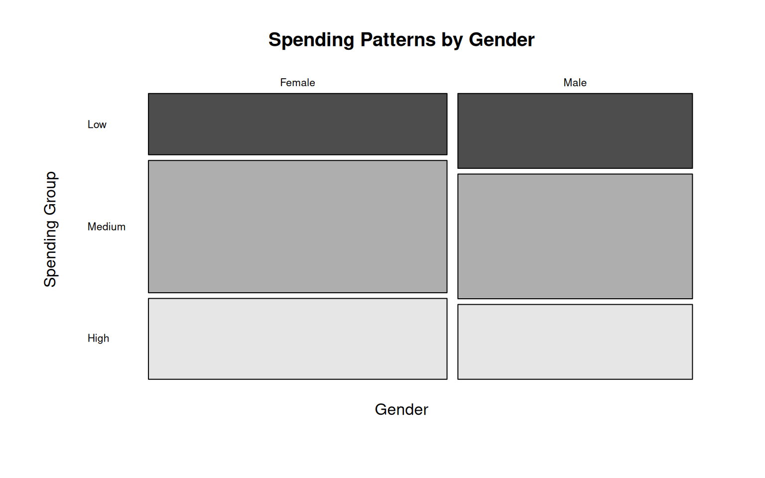
# Create contingency table: Gender vs Spending Groupgender_spending_table <-table(mall_data$Genre, mall_data$Spending_Group)print("Gender vs Spending Group Contingency Table:")
# Visualize the relationshipmosaicplot(gender_spending_table,main ="Spending Patterns by Gender",color =TRUE,las =1,xlab ="Gender",ylab ="Spending Group")
# Create another table: Income Group vs Spending Groupincome_spending_table <-table(mall_data$Income_Group, mall_data$Spending_Group)print("Income Group vs Spending Group Contingency Table:")
[1] "Income Group vs Spending Group Contingency Table:"
print(income_spending_table)
             Low Medium High
  Low         12      6   14
  Medium-Low   5     56    5
  Medium      22     31   27
  High        10      1   11
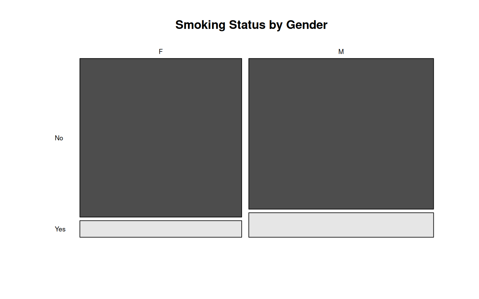
# Create contingency table: Gender vs Smoking Statusgender_smoke_table <-table(student_data$Gender, student_data$Smoke)print("Gender vs Smoking Status Contingency Table:")
    Pearson's Chi-squared test with Yates' continuity correction

data:  gender_smoke_table
X-squared = 1.3548, df = 1, p-value = 0.2444
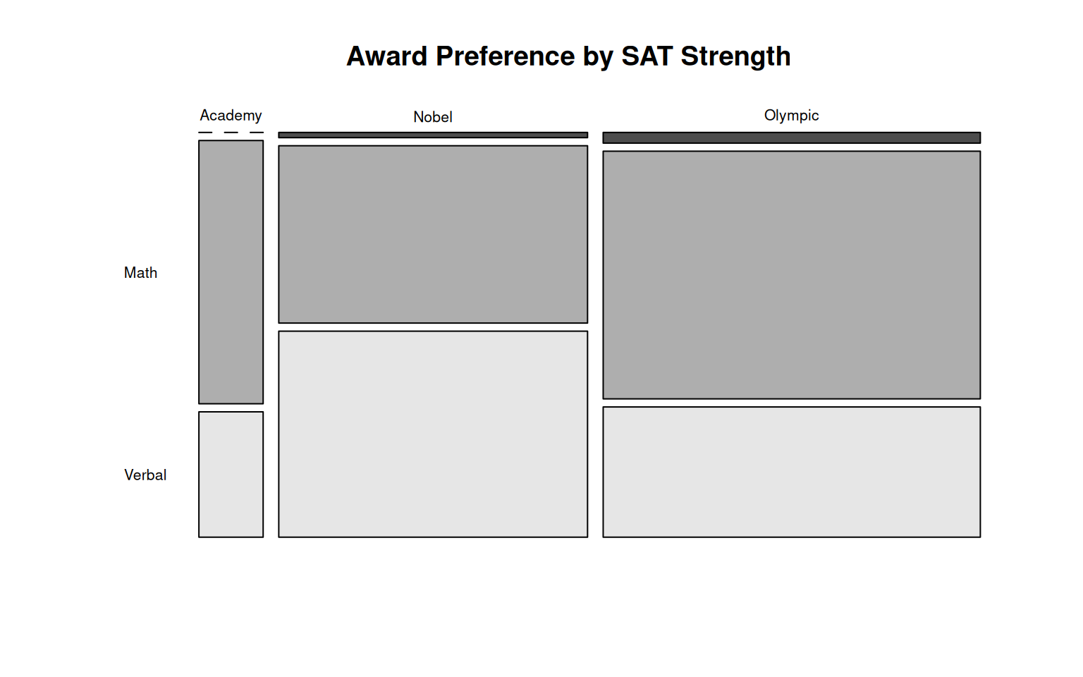
# Create table: Award Preference vs Higher SATaward_sat_table <-table(student_data$Award, student_data$HigherSAT)print("Award Preference vs Higher SAT Contingency Table:")
[1] "Award Preference vs Higher SAT Contingency Table:"
print(award_sat_table)
              Math Verbal
  Academy   0   21     10
  Nobel     2   68     79
  Olympic   5  116     61
# Visualize relationshipsmosaicplot(gender_smoke_table,main ="Smoking Status by Gender",color =TRUE,las =1)
mosaicplot(award_sat_table,main ="Award Preference by SAT Strength",color =TRUE,las =1)
Part 3: Goodness-of-Fit Testing
3.1 Mall Customer Distribution Analysis
# Test if gender distribution is equal (50/50)observed_gender <-table(mall_data$Genre)print("Observed Gender Distribution:")
[1] "Observed Gender Distribution:"
print(observed_gender)
Female   Male
   112     88
# Expected distribution: equal proportionschi_gender_fit <-chisq.test(observed_gender, p =c(0.5, 0.5))print("Goodness-of-Fit Test for Gender Distribution:")
[1] "Goodness-of-Fit Test for Gender Distribution:"
print(chi_gender_fit)
    Chi-squared test for given probabilities

data:  observed_gender
X-squared = 2.88, df = 1, p-value = 0.08969
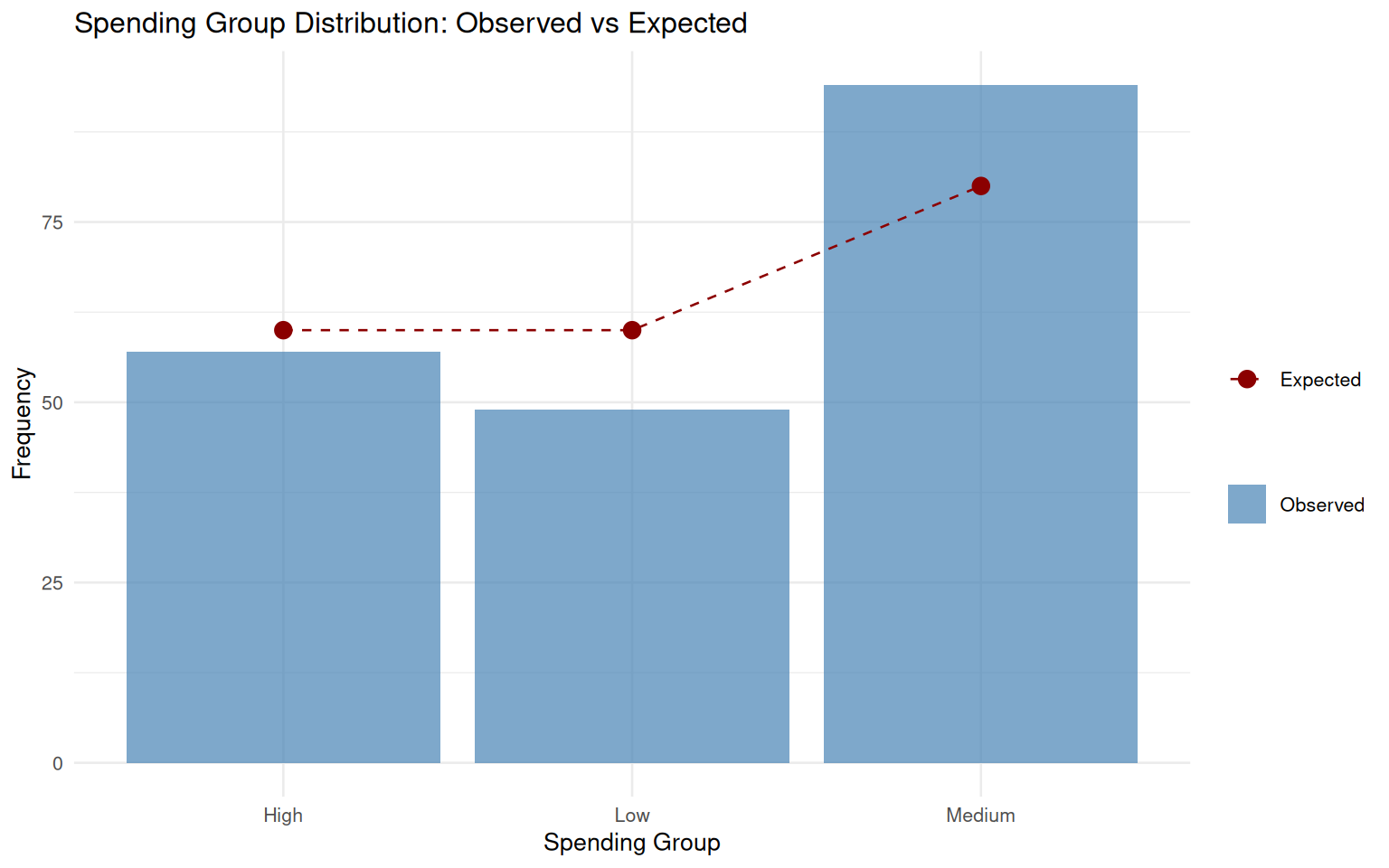
# Test if spending groups follow specific distributionobserved_spending <-table(mall_data$Spending_Group)print("Observed Spending Group Distribution:")
[1] "Observed Spending Group Distribution:"
print(observed_spending)
   Low Medium   High
    49     94     57
# Expected distribution: 30% Low, 40% Medium, 30% Highexpected_proportions <-c(0.3, 0.4, 0.3)chi_spending_fit <-chisq.test(observed_spending, p = expected_proportions)print("Goodness-of-Fit Test for Spending Groups:")
[1] "Goodness-of-Fit Test for Spending Groups:"
print(chi_spending_fit)
    Chi-squared test for given probabilities

data:  observed_spending
X-squared = 4.6167, df = 2, p-value = 0.09943
# Visualize observed vs expectedspending_df <-tibble(Group =names(observed_spending),Observed =as.numeric(observed_spending),Expected =sum(observed_spending) * expected_proportions)ggplot(spending_df, aes(x = Group)) +geom_bar(aes(y = Observed, fill ="Observed"), stat ="identity", alpha =0.7) +geom_point(aes(y = Expected, color ="Expected"), size =3) +geom_line(aes(y = Expected, color ="Expected", group =1), linetype ="dashed") +labs(title ="Spending Group Distribution: Observed vs Expected",y ="Frequency", x ="Spending Group") +scale_fill_manual("", values ="steelblue") +scale_color_manual("", values ="darkred") +theme_minimal(base_size =10)
3.2 Student Survey Distribution Analysis
# Test if award preferences are equally distributedobserved_awards <-table(student_data$Award)print("Observed Award Preferences:")
[1] "Observed Award Preferences:"
print(observed_awards)
Academy   Nobel Olympic
     31     149     182
# Expected: equal distribution among three awardsexpected_award_proportions <-c(1/3, 1/3, 1/3)chi_award_fit <-chisq.test(observed_awards, p = expected_award_proportions)print("Goodness-of-Fit Test for Award Preferences:")
[1] "Goodness-of-Fit Test for Award Preferences:"
print(chi_award_fit)
    Chi-squared test for given probabilities

data:  observed_awards
X-squared = 104.46, df = 2, p-value < 2.2e-16
# Test if smoking status follows population distributionobserved_smoking <-table(student_data$Smoke)print("Observed Smoking Status:")
[1] "Observed Smoking Status:"
print(observed_smoking)
 No Yes
319  43
# Expected: 80% non-smokers, 20% smokers (based on general population)# table() orders levels alphabetically as No, Yesexpected_smoking_proportions <-c(No =0.8, Yes =0.2)chi_smoking_fit <-chisq.test(observed_smoking, p = expected_smoking_proportions)print("Goodness-of-Fit Test for Smoking Status:")
[1] "Goodness-of-Fit Test for Smoking Status:"
print(chi_smoking_fit)
    Chi-squared test for given probabilities

data:  observed_smoking
X-squared = 14.923, df = 1, p-value = 0.000112
Assessment (Total: 50 points)
Section A: Formative Understanding (15 points)
A1. Explain the difference between chi-square test of independence and chi-square goodness-of-fit test. When would you use each type of test? Provide concrete examples for both. (4 points)
A2. Describe the key assumptions for chi-square tests and explain why the “expected counts ≥ 5” condition is important. What should you do when this condition is violated? (4 points)
A3. Write the null and alternative hypotheses for both a test of independence and a goodness-of-fit test. Explain how the interpretation differs between these two types of tests. (4 points)
A4. Discuss the role of contingency tables in chi-square analysis. How do you calculate expected frequencies, and what do they represent in the context of hypothesis testing? (3 points)
Section B: Application and Analysis (20 points)
B1. Test whether there is a relationship between gender and spending patterns in the mall customers dataset using α = 0.05. Create the appropriate contingency table, check assumptions, perform the chi-square test, and interpret your results. (5 points)
# Create contingency table
B2. Test whether income group and spending group are independent in the mall customers dataset using α = 0.05. Conduct the appropriate analysis and discuss whether the relationship makes practical sense. (5 points)
# Create contingency table
B3. Test whether gender and smoking status are independent in the student survey dataset using α = 0.05. Create the contingency table, check assumptions, and interpret your findings in the context of college student behavior. (5 points)
# Create contingency table
B4. Conduct a goodness-of-fit test to determine if award preferences in the student survey follow an equal distribution among the three options (Nobel Prize, Olympic Gold, Academy Award) using α = 0.05. Interpret your results. (5 points)
# Get observed frequencies
Section C: Statistical Synthesis (15 points)
C1. Create a comprehensive decision framework (200-250 words) for selecting appropriate categorical data analysis methods. Include guidance on when to use chi-square tests of independence, goodness-of-fit tests, and alternative methods like Fisher’s exact test. (7 points)
C2. Design a research study that would require chi-square analysis. Describe the categorical variables, research question, expected sample size, and how you would ensure assumptions are met. Include potential limitations and how you would address them. (4 points)
C3. Compare and contrast the mall customers dataset analysis with the student survey dataset analysis. Discuss the different types of relationships you might expect to find in these two contexts and how the interpretation of results would differ. (4 points)
Submission Guidelines:
Complete R Markdown document with all code and analysis
Proper execution of all chi-square tests following appropriate procedures
Comprehensive assumption checks with expected frequency analysis
Professional writing with clear analytical narrative and interpretation
Appropriate test justifications based on data characteristics
Knitted HTML document submitted via designated platform